2D dynamic: temporal TV
This example illustrates 2D dynamic MRI image reconstruction from golden angle (GA) radial sampled k-space data collected with multiple coils (parallel MRI), with temporal "TV" regularizer (corner-rounded) using the Julia language.
This page comes from a single Julia file: 3-2d-t.jl.
You can access the source code for such Julia documentation using the 'Edit on GitHub' link in the top right. You can view the corresponding notebook in nbviewer here: 3-2d-t.ipynb, or open it in binder here: 3-2d-t.ipynb.
using ImageGeoms: ImageGeom
using ImagePhantoms: shepp_logan, SouthPark, phantom, ellipse, spectrum
using MIRTjim: jim, prompt
using MIRT: Anufft, diffl_map, ncg
using MIRT: ir_mri_sensemap_sim, ir_mri_kspace_ga_radial
using Plots: gui, plot, scatter, default; default(markerstrokecolor=:auto, label="")
using Plots: gif, @animate, Plots
using LinearAlgebra: norm, dot, Diagonal
using LinearMapsAA: LinearMapAA, block_diag
using Random: seed!
jim(:abswarn, false); # suppress warnings about display of |complex| images
The following line is helpful when running this jl-file as a script; this way it will prompt user to hit a key after each image is displayed.
isinteractive() && jim(:prompt, true);Define dynamic image sequence
N = (60,64)
fov = 220
nt = 8 # frames
ig = ImageGeom(; dims = N, deltas=(fov,fov) ./ N)

object0 = shepp_logan(SouthPark(); fovs = (fov,fov))
objects = Array{typeof(object0)}(undef, nt)
xtrue = Array{ComplexF32}(undef, N..., nt)
for it in 1:nt
    tmp = copy(object0)
    width2 = 15 + 5 * sin(2π*it/nt) # mouth open/close
    mouth = tmp[2]
    tmp[2] = ellipse(mouth.center, (mouth.width[1], width2), mouth.angle[1], mouth.value)
    objects[it] = tmp
    xtrue[:,:,it] = phantom(axes(ig)..., tmp, 4)
end
jimxy = (args...; aspect_ratio=1, kwargs...) ->
    jim(axes(ig)..., args...; aspect_ratio, kwargs...)
jimxy(xtrue, "True images"; nrow=2)
Animate true image:
anim1 = @animate for it in 1:nt
    jimxy(xtrue[:,:,it], title="Frame $it")
end
gif(anim1; fps = 6)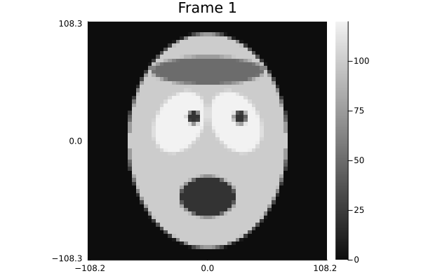
Plot one time course to see temporal change:
ix,iy = 30,14
plot(1:nt, abs.(xtrue[ix,iy,:]), label="ix=$ix, iy=$iy",
    marker=:o, xlabel="frame")
isinteractive() && prompt();Define k-space sampling
accelerate = 3
nspf = round(Int, maximum(N)/accelerate) # spokes per frame

Nro = maximum(N)
Nspoke = nspf * nt
kspace = ir_mri_kspace_ga_radial(; Nro, Nspoke)
fovs = (fov, fov)
kspace[:,:,1] ./= fovs[1]
kspace[:,:,2] ./= fovs[2]
kspace = reshape(kspace, Nro, nspf, nt, 2)
(size(kspace), extrema(kspace))
((64, 21, 8, 2), (-0.0022727272f0, 0.002272619f0))Plot sampling (in units of cycles/pixel):
ps = Array{Any}(undef, nt)
for it in 1:nt
    ps[it] = scatter(kspace[:,:,it,1] * fovs[1], kspace[:,:,it,2] * fovs[2],
        xtick=(-1:1)*0.5, ytick=(-1:1)*0.5, xlim=(-1,1).*0.5, ylim=(-1,1).*0.5,
        aspect_ratio=1, markersize=1, title="Frame $it", widen=true)
end
plot(ps...; layout=(2,4))
isinteractive() && prompt();

anim2 = @animate for it in 1:nt
    plot(ps[it])
end
gif(anim2; fps = 6)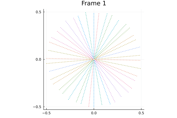
Make sensitivity maps, normalized so SSoS = 1:
ncoil = 2
smap_raw = ir_mri_sensemap_sim(dims=N, ncoil=ncoil, orbit_start=[90])
p1 = jim(smap_raw, "Sensitivity maps raw");

sum_last = (f, x) -> selectdim(sum(f, x; dims=ndims(x)), ndims(x), 1)
ssos_fun = smap -> sqrt.(sum_last(abs2, smap)) # SSoS
ssos_raw = ssos_fun(smap_raw)
p2 = jim(ssos_raw, "SSoS for ncoil=$ncoil");

smap = smap_raw ./ ssos_raw
p3 = jim(smap, "Sensitivity maps");

ssos = ssos_fun(smap) # SSoS
@assert all(≈(1), ssos)
jim(p1, p2, p3)
System matrix
Make system matrix for dynamic non-Cartesian parallel MRI:
Fs = Array{Any}(undef, nt)
for it in 1:nt # a NUFFT object for each frame
    Ω = [kspace[:,:,it,1][:] kspace[:,:,it,2][:]] * fov * 2pi
    Fs[it] = Anufft(Ω, N, n_shift = [N...]/2)
end
Block diagonal system matrix, with one NUFFT per frame
S = [Diagonal(vec(selectdim(smap, ndims(smap), ic))) for ic in 1:ncoil]
SO = s -> LinearMapAA(s ; idim=N, odim=N) # LinearMapAO for coil maps
AS1 = F -> vcat([F * SO(s) for s in S]...); # [A1*S1; ... ; A1*Sncoil]
Linear operator input is (N..., nt), output is (nspf*Nro, Ncoil, nt)
A = block_diag([AS1(F) for F in Fs]...) # todo: refine show()
(size(A), A._odim, A._idim)
((21504, 30720), (1344, 2, 8), (60, 64, 8))Simulate k-space data via an inverse crime (todo):
ytrue = A * xtrue
snr2sigma = (db, yb) -> # compute noise sigma from SNR (no sqrt(2) needed)
    10^(-db/20) * norm(yb) / sqrt(length(yb))
sig = Float32(snr2sigma(50, ytrue))
seed!(0)
y = ytrue + sig * randn(ComplexF32, size(ytrue))
ysnr = 20*log10(norm(ytrue) / norm(y - ytrue)) # verify SNR50.01468271839975Initial image
Initial image via zero-fill and scaling: todo: should use density compensation, perhaps via VoronoiDelaunay.jl
x0 = A' * y # zero-filled recon (for each frame)
tmp = A * x0 # (Nkspace, Ncoil, Nframe)
x0 = (dot(tmp,y) / norm(tmp)^2) * x0 # scale sensibly
jimxy(x0, "initial image"; nrow=2)
Temporal finite differences:
Dt = diffl_map((N..., nt), length(N)+1 ; T=eltype(A))
tmp = Dt' * (Dt * xtrue)
jimxy(tmp, "Time differences are sparse"; nrow=2)
Regularized CG reconstruction
Run nonlinear CG on "temporal edge-preserving" regularized LS cost function
niter = 90
delta = Float32(0.1) # small relative to temporal differences
reg = Float32(2^20) # trial and error here
ffair = (t,d) -> d^2 * (abs(t)/d - log(1 + abs(t)/d))
pot = z -> ffair(z, delta)
dpot = z -> z / (Float32(1) + abs(z/delta))
cost = x -> 0.5 * norm(A*x - y)^2 + reg * sum(pot.(Dt * x))
fun = (x,iter) -> cost(x)
gradf = [v -> v - y, u -> reg * dpot.(u)]
curvf = [v -> Float32(1), u -> reg]
(xh, out) = ncg([A, Dt], gradf, curvf, x0 ; niter, fun)
costs = [out[i+1][1] for i=0:niter];
Show results
pr = plot(
    jimxy(xtrue, "|xtrue|"; nrow=2),
    jimxy(xh, "|recon|"; nrow=2),
    jimxy(xh-xtrue, "|error|"; nrow=2),
    scatter(0:niter, log.(costs), label="cost", xlabel="iteration"),
)
isinteractive() && prompt();Animate true, recon, error
anim3 = @animate for it in 1:nt
    plot(
        jimxy(xtrue[:,:,it], clim=(0,120), title="True"),
        jimxy(xh[:,:,it], clim=(0,120), title="|Recon|"),
        jimxy(xh[:,:,it] - xtrue[:,:,it], clim=(0,30), title="|Error|"),
        plot_title = "Frame $it",
        layout = (1,3),
    )
end
gif(anim3; fps = 6)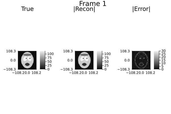
This page was generated using Literate.jl.